Normal Modes, Eigenvectors -

Introduction

In this article, We show that important concepts in system theory like poles and normal modes follow directly from the mathematical structural of the dynamic equation $\dot{\mathbf{x}}=\mathbf{A}\mathbf{x}$ . This conceptualization is very helpful. It provides a general framework that can describe a multitude of systems and phenomena as long as they can be explained by the dynamic equation. It also establishes the connection between physics and mathematical spaces that is very important in Quantum mechanics.

From state variables to state vector

An $n^\textnormal{th}$ order differential equation can be represented by a system of $n$ first order differential equations in the variables $x_1, x_2,\cdots, x_n$ which we have called the state variables. It is very helpful to consider such variables as the components of a state vector $\mathbf{x}=[x_1, x_2, \cdots, x_n]^t$ . This vector lives in the mathematical space $\mathbb{C}^n$ .

The main idea of normal modes is related to realizing that $\mathbf{x}$ being a vector is an entity that transcends its representation. We then seek appropriate coordinate systems (basis in the language of linear algebra) that simplifies the analysis. This is where normal modes or equivalently the concept of eigenvectors become very important.

Changing the basis

First lets consider the homogeneous case. We have already shown that

(1) $\begin{equation*} \mathbf{x}(t)=e^{t\mathbf{A}}\mathbf{x}(0). \end{equation*}$

Changing the coordinates in $\mathbb{C}^n$ is equivalent to matrix multiplication. Therefore we change from the natural basis where the components of $\mathbf{x}$ is $x_1, x_2,\cdots, x_n$ to another basis $\{e_1, e_2,\cdots, e_n\}$ where the components of $\mathbf{x}$ are $x_1',x_2',\cdots , x_n'$ via the transformation matrix $S$ :

(2) $\begin{equation*} \mathbf{x}=S\mathbf{x'}. \end{equation*}$

Plugging in the previous equation, one can find that

(3) $\begin{equation*} \mathbf{x}'(t)=S^{-1}e^{t\mathbf{A}}S\mathbf{x'}(0). \end{equation*}$

Now $S^{-1}e^{t\mathbf{A}}S$ is the representation of the transformation operator in the new basis. Such transformation is called similarity transformation. An important property of the exponential matrix is that:

(4) $\begin{equation*} S^{-1}e^\mathbf{A}S= e^{S^{-1}\mathbf{A}S}. \end{equation*}$

An important basis are the ones that make $\mathbf{A}$ diagonal. In this particular basis each component $x_k'$ of $\mathbf{x}'$ at time $t$ is related to the same component $x_k'(0)$ via a multiplication operation and is basically uncoupled from other components $j\neq k$ . These particular basis are called the eigenvectors of $\mathbf{A}$ . In this case

(5) $\begin{align*} \begin{bmatrix} x_1'(t)\\ x_2'(t) \\ \cdots \\ x_{n-1}'(t)\\ x_n'(t) \end{bmatrix} &=\begin{bmatrix} e^{a_1t} &0 &0 &0 &0\\ 0 &e^{a_2t} & 0 &0 &0\\ \vdots & \cdots &\ddots & \cdots &\vdots\\ 0 & \cdots & 0 & e^{a_{n-1}t} &0\\ 0 &\cdots & 0 & 0 & e^{a_nt} \end{bmatrix} \begin{bmatrix} x_1'(0)\\ x_2'(0) \\ \cdots \\ x_{n-1}'(0)\\ x_n'(0) \end{bmatrix}\\ &=\begin{bmatrix} x_1'(0)e^{a_1t}\\ x_2'(0)e^{a_2t} \\ \cdots \\ x_{n-1}'(0)e^{a_{n-1}t}\\ x_n'(0)e^{a_nt} \end{bmatrix} \end{align*}$

Here $a_k$ is the $k^\textnormal{th}$ eigenvalue or pole of $\mathbf{A}$ . (We assume that eigenvalues are simple, i.e, all eigenvalues are different).

If we denote the $k^\textnormal{th}$ eigenvector by $\mathbf{v}_k$ then the transformation $S$ can be written as

(6) $\begin{equation*} S=\begin{bmatrix} \mathbf{v}_1 &\mathbf{v}_2 &\cdots &\mathbf{v}_{n-1} &\mathbf{v}_n \end{bmatrix}, \end{equation*}$

where

(7) $\begin{equation*} \mathbf{v}_k=\begin{bmatrix} v_{k1} \\ v_{k2} \\ \vdots \\ v_{kn-1} \\ v_{kn} \end{bmatrix} \end{equation*}$

is the components of the $k^\textnormal{th}$ in the original coordinate system.

To conclude: the $k^\textnormal{th}$ normal mode is represented by the eigenvector $\mathbf{v}_k$ and the eigenvalue $e^{a_kt}$ and it evolves as

$x'_k(0)e^{a_kt}\mathbf{v}_k.$

This means that all components of $\mathbf{v}_k$ evolve in the same way. For harmonic (oscillating) systems, $a_k$ is complex and represents a damped oscillation. In this case, all components of the state vector oscillates with the same frequency.

Example: un-damped LC resonator

To demonstrate the process described above, I show here an example of a simple LC circuit, which is formed by an inductor and a capacitor.

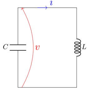
LC resonator

For the LC circuit shown above,

$\begin{align*} v&=L\frac{di}{dt}\\ i&=C\frac{dv}{dt} \end{align*}$

If we define $x_1$ to be $v$ and $x_2$ to be $i$ then we can write

(8) $\begin{equation*} \underbrace{\begin{bmatrix} \dot{x}_1 \\ \dot{x}_2 \end{bmatrix}}_{\dot{\mathbf{x}}} =\underbrace{\begin{bmatrix} 0 & 1/C \\ 1/L & 0 \end{bmatrix}}_{\mathbf{A}} \underbrace{\begin{bmatrix} {x}_1 \\ {x}_2 \end{bmatrix}}_{\mathbf{x}}. \end{equation*}$

Using linear algebra, eigenvalues of $\mathbf{A}$ can be found to $\lambda=\pm j\omega_0$ where

$\omega_0=\frac{1}{\sqrt{LC}}.$

Additionally the eigenvectors are found to be

(9) $\begin{equation*} \mathbf{v}_\pm= \frac{1}{\sqrt{1+Z_0^2}}\begin{bmatrix} \mp jZ_0 \\ 1 \end{bmatrix}, \end{equation*}$

where

$Z_0\triangleq \sqrt{\frac{L}{C}}.$

Therefore,

(10) $\begin{equation*} \frac{1}{\sqrt{1+Z_0^2}}\begin{bmatrix} \mp jZ_0 \\ 1 \end{bmatrix} e^{\pm j\omega t} \end{equation*}$

represent the normal modes. In fact each vector is the complex conjugate of the other; hence they both represent the same mode. It is clear that the mode components oscillate with the same frequency $\omega_0$ , which we will call it the resonant frequency. But what does each vector component represent?

The first component of either $\mathbf{v}_+$ or $\mathbf{v}_-$ represents the state variable $x_1$ (or $v$ ). The second component represents $x_2$ (or $i$ ). Therefore,

$v=\mp jZ_0 i= \mp j\sqrt{\frac{L}{C}}i$

Multiplying both sides by $\omega_0$ one gets

$v=\pm \frac{1}{j\omega_0 C} i,$

which is what we expect from circuit theory.

Exercise

Include a series resistor and calculate the eigenvectors and eigenvalues and find expressions for the normal modes (eigenvalues in this case will be complex, i.e, the mode loses energy over time due to the dissipation effect of the resistor).

A challenging exercise

(If you solved it, please send me the solution and I will include it under YOUR name. I will only publish the most complete answer.)

The following coupled LC circuit. This circuit represents a wireless power transfer system that exploits resonance to efficiently transfer power.

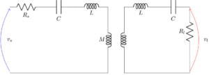
Inductive coupling between two LC resonators.

Find

The system matrix $\mathbf{A}$ .
The eigenvalues and eigenvector of $\mathbf{A}$ . (you should get a symmetric and anti-symmetric eigenvector. The eigenvalues will be two resonant frequencies that will change from $\omega_0=1/\sqrt{LC}$ to something other value that also depends on $M$ ).
The normal modes.
(optional) If $v_s$ and $v_l$ are the input and output voltages respectively, find the matrices $\mathbf{B}$ and $\mathbf{C}$ .