Systems: State Space and Convolution Representations -

Introduction

Physical systems are described by differential equations. Newton’s second law, Electromagnetism, Circuits and Schrodinger’s equations are just a few examples. Differential equations are defined by their order: the highest derivative. Additionally a differential equation of some order $n$ can be converted to a system of $n$ first order coupled differential equations and in general can be written as

(1) $\begin{equation*} \frac{d\mathbf{x}}{dt}=f(\mathbf{x},\mathbf{u}) \end{equation*}$

(2) $\begin{equation*} \mathbf{y}=g(\mathbf{x}), \end{equation*}$

where $\mathbf{x}$ is a $n$ long vector known as the state vector, $\mathbf{u}$ is the input vector (for example think of a muliport network that can be excited by applying voltages to its inputs. $\mathbf{y}$ is the system output, which is a function of $\mathbf{x}$ .

For many electrical engineering applications, the system of differential equations is built from the relations between current and voltages ( $v=Ri,~i=Cdv/dt,~ v=Ldi/dt$ ). $R$ , $C$ and $L$ are almost always linear and do not change with time (time invariant). For circuits (and many other engineering systems) (1) takes the form

(3) $\begin{equation*} \frac{d\mathbf{x}}{dt}=\mathbf{A}\mathbf{x}+\mathbf{B}\mathbf{u} \end{equation*}$

and

(4) $\begin{equation*} \mathbf{y}=\mathbf{C}\mathbf{x}, \end{equation*}$

where now $\mathbf{A},~\mathbf{B}$ and $\mathbf{C}$ are matrices.

Although the laws of physics in the language of differential equations, they have been obtained from observing and measuring quantities over short but non-infinitesimal intervals of times. Therefore, it is sometimes useful to go back from the differential equations to the underlying difference system of equations. Now instead of talking about instantaneous rate of changes, we talk about average rates. Integrating (3) over some time interval $\Delta t=t_2-t_1$ leads to

(5) $\begin{equation*} \Delta \mathbf{x}=\mathbf{x}_2-\mathbf{x}_1=\mathbf{A}\bar{\mathbf{x}}\Delta t+\mathbf{B}\bar{\mathbf{u}}\Delta t. \end{equation*}$

In the above equation $\bar{\mathbf{x}}$ and $\bar{\mathbf{u}}$ are the average values of $\mathbf{x}$ and $\mathbf{u}$ over $\Delta t$ . If $\mathbf{x}$ and $\mathbf{u}$ are sufficiently smooth function then

(6) $\begin{equation*} \bar{\mathbf{x}}=\mathbf{x}(t_m)+O^2(\Delta t)=\frac{\mathbf{x}_1+\mathbf{x}_2}{2}+O^2(\Delta t), \end{equation*}$

(7) $\begin{equation*} \bar{\mathbf{u}}=\mathbf{u}(t_{mid})+O^2(\Delta t)=\frac{\mathbf{u}_1+\mathbf{u}_2}{2}+O^2(\Delta t), \end{equation*}$

where $t_{mid}=0.5(t_1+t_2)$ . Therefore (5) becomes

(8) $\begin{equation*} \mathbf{x}_2=\left(\mathbf{I}-\frac{\Delta t}{2}\mathbf{A})\right)^{-1}\left(\mathbf{I}+\frac{\Delta t}{2}\mathbf{A})\right)\mathbf{x}_1+\left(\mathbf{I}-\frac{\Delta t}{2}\mathbf{A})\right)^{-1}\mathbf{B}\mathbf{u}(t_{mid})\Delta t +O^2(\Delta t). \end{equation*}$

Rendered by QuickLaTeX.com

In general if we know an initial state $\mathbf{x}_0$ at time $t=0$ then we divide the interval $[0,t]$ into $n$ sub-intervals with an increment of $\Delta t=t/n$ (see the figure above). This allows us +(in principle) to find $x$ at $t$ . In general if we labelled the state vector at each time instant by the increment $i=0, 1, 2,\cdots n$ then

(9) $\begin{equation*} \mathbf{x}_n=\underbrace{\left(\mathbf{I}-\frac{\Delta t}{2}\mathbf{A})\right)^{-1}\left(\mathbf{I}+\frac{\Delta t}{2}\mathbf{A})\right)}_{{\textnormal{Homogeneous}}}\mathbf{x}_{n-1}+\underbrace{\left(\mathbf{I}-\frac{\Delta t}{2}\mathbf{A})\right)^{-1}\mathbf{B}\mathbf{u}_{n-1/2}\Delta t}_{{\textnormal{Nonhomogeneous}}} +O^2(\Delta t), \end{equation*}$

where now $\mathbf{u}$ is calculated at $t_{n-1/2}$ : the mid point of the interval $[t_{n-1} ~t_n]$ . For simplicity we define $\mathbf{\Phi}$ and $\mathbf{G}$ to be

(10) $\begin{equation*} \mathbf{\Phi}\triangleq \left(\mathbf{I}-\frac{\Delta t}{2}\mathbf{A})\right)^{-1}\left(\mathbf{I}+\frac{\Delta t}{2}\mathbf{A})\right) \end{equation*}$

and

(11) $\begin{equation*} \mathbf{G}\triangleq \left(\mathbf{I}-\frac{\Delta t}{2}\mathbf{A})\right)^{-1}\mathbf{B}. \end{equation*}$

This means that we can write (9) in terms of the newly defined matrices as

(12) $\begin{equation*} \mathbf{x}_n=\mathbf{\Phi}\mathbf{x}_{n-1}+\mathbf{G}\mathbf{u}_{n-1/2}\Delta t+O^2(\Delta t) \end{equation*}$

Evolution of the state vector over time.

Equation (12) and the Figure above reveals the mechanism at which the state vector $\mathbf{x}_n$ evolves over time. $\mathbf{x}_n$ evolves from the previous state $\mathbf{x}_{n-1}$ through two basic linear operations: (1) Linearly transforming the state $\mathbf{x}_{n-1}$ by the application of the linear operator $\mathbf{\Phi}$ and in addition (2) the linear mapping of the input vector $\mathbf{u}$ and the event $t-\Delta t/2$ .

As we will see later, the two transformations mainly depend on the properties of the system matrix $\mathbf{A}$ . In the next section, the input is turned off (i.e, $\mathbf{u}=\mathbf{0}$ ). Therefore we will be interested in the behaviour of the matrix $\mathbf{\Phi}$ .

Homogeneous case: $\mathbf{u}=\mathbf{0}$

In this case

(13) $\begin{equation*} \mathbf{x}_n=\mathbf{\Phi}\mathbf{x}_{n-1} \end{equation*}$

(14) $\begin{equation*} \mathbf{x}_n=\mathbf{\Phi}^n\mathbf{x}_{0} \end{equation*}$

We Let $n=2n'$ , $n'=1,2,\cdots$ . We also note that the \textbf{exponential} of a matrix $e^\mathbf{X}$ is defined to be

(15) $\begin{equation*} e^\mathbf{X}=\lim_{N\rightarrow~\infty}\left(\mathbf{I}+\frac{1}{N}\mathbf{X}\right)^N, \end{equation*}$

For our purposes it is sufficient to say that such matrix sequence converges. Therefore, if we divide the time interval $[0~t]$ into an infinitely many sub-intervals one gets ( $\mathbf{G}^n$ approaches $e^{t\mathbf{A}}$ as $n$ increases).

(16) $\begin{equation*} \mathbf{x}(t)=e^{t\mathbf{A}}\mathbf{x}(0). \end{equation*}$

Nonhomogeneous case, $\mathbf{u}\neq \mathbf{0}$

In this case we use the general form (9) and apply it iteratively at the time steps $n, n-1,\cdots, 0$ . Note that at each time step $\mathbf{x}_n$ depends on the previous value $\mathbf{x}_{n-1}$ and $\mathbf{u}_{n-1/2}$ . This means that $\mathbf{x}_n$ depends on $\mathbf{x}_0$ and \emph{all} previous inputs $\mathbf{u}$ at $n-1/2, n-3/2,\cdots, 1/2$ . The dependency of $\mathbf{x}_n$ on all the previous input values is nothing but the \textbf{convolution} operation. In fact it is easy to show that

(17) $\begin{equation*} \mathbf{x}_n=\mathbf{\Phi}^n\mathbf{x}_{0}+\sum_{i=1}^n \mathbf{\Phi}^{i-1}\mathbf{G}\mathbf{u}_{n+1/2-i}. \end{equation*}$

Note that

$\left[\left(\mathbf{I}-\frac{\Delta t}{2}\mathbf{A})\right)^{-1}\left(\mathbf{I}+\frac{\Delta t}{2}\mathbf{A})\right)\right]^{i-1}=e^{\tau_i\mathbf{A}}+\underbrace{O^i(\Delta t)}_\textnormal{remainder}.$

Therefore (17) becomes

(18) $\begin{equation*} \mathbf{x}_n=e^{t\mathbf{A}}\mathbf{x}_{0}+\underbrace{\Delta t\sum_{i=1}^ne^{\tau_i\mathbf{A}}\mathbf{B}\mathbf{u}_{n+1/2-i}}_\textnormal{{Riemann sum}}+\underbrace{\Delta t\sum_{i=1}^n O^i(\Delta t)\left(\mathbf{I}-\frac{\Delta t}{2}\mathbf{A})\right)^{-1}\mathbf{B}\mathbf{u}_{n+1/2-i}+O^{n+1}(\Delta t)}_\textnormal{higher order}. \end{equation*}$

Note that $\mathbf{u}$ above is sampled at the points $(n-i+1/2)\Delta t=t-\tau_i+\Delta t/2$ .

If we divide the interval $[0,~t]$ to infinitely many sub-intervals, i.e, letting $n\rightarrow~\infty$ . Therefore,

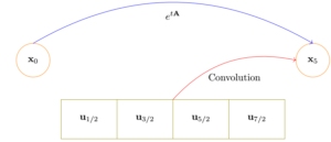
(19) $\begin{equation*} \mathbf{x}(t)=e^{t\mathbf{A}}\mathbf{x}(0)+\int_0^t e^{\tau\mathbf{A}}\mathbf{B}\mathbf{u}(t-\tau)d\tau \end{equation*}$

Convolution operator maps the inputs to the states.

The figure above shows how the state at final time $\mathbf{x}_5$ is related to the initial state $\mathbf{x}_0$ and the history of the input $\mathbf{u}$ . This is the convolution picture, where the dependency on the states has been encapsulated in the convolution operation.