Maxwell’s equations in 2D
Consider a system that is infinitely long in the  direction such that
  . Therefore Maxwell’s equations reduce to
(1) 
(2) 
 is the 2D curl operation, which is equal to
(3) 
Note that in the 2D case, Maxwell’s equations split into two decoupled systems as shown by the above two systems of equations. The first (second) system is called the TM (TE) mode since  (
( ).
).
Wave Equation
For the TM mode, we can eliminate the magnetic field  to get the wave equation
(4) 
where
![\[\nabla_{2D}^2 P=\partial_x^2 P+\partial_y^2 P.\]](http://samehelnaggar.ca/wp-content/ql-cache/quicklatex.com-1f47cc436f56643a6b3efe5ba2f7ffef_l3.png "Rendered by QuickLaTeX.com")
Similarly the wave equation of the TE assumes the form
(5) 
Normal (eigen) modes
When the source term  or
or  is zero then we end up with the homogeneous wave equation:
(6) 
If we consider fields that sinusoidally vary with time (i.e.,  ) then we end up with the following eigenvalue problem
(7) 
If we consider the structure to be an infinitely long with a rectangular cross section as shown below, where the orange lines represent conducting boundaries. For the TM mode this means that:

\centering

It can shown that for the TM mode,  can be written as
(8) 
where
![\[K_x=\frac{m\pi}{a}\]](http://samehelnaggar.ca/wp-content/ql-cache/quicklatex.com-dcce0506fea53acb63864d2b4a9aab58_l3.png "Rendered by QuickLaTeX.com")
,
![\[K_y=\frac{n\pi}{b}.\]](http://samehelnaggar.ca/wp-content/ql-cache/quicklatex.com-a46913f0e75cf56c53ad137ce18aa07c_l3.png "Rendered by QuickLaTeX.com")
where  is the mode number. A mode is identified by its mode number. Therefore it is convenient to write the mode as
  , which has a resonant frequency:
(9) 
where again I used the normalized unit ( ). I also considered the case where the cavity is filled with air. The figure below plots the fields of the first 20 modes (
 ).
).
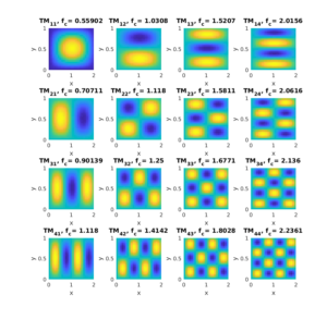
The electric field of the first 16 TM modes.
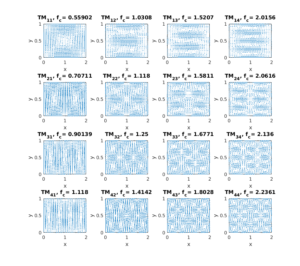
The magnetic field of the first 16 TM modes.
Mode Excitation
For this animation, I made the cross section to be square. In the first case the length of the square was set to  to make sure that the resonant frequency of the
  mode is 1 unit. In the second example, the length was changed to
  such that the resonant frequency of the
  or
or  modes to be unity.
Note that the mode strength increases as the source approached the center of the cavity. By inspecting the profile of the magnetic field of the TM11 mode shown below, it is clear that the magnetic fields “circulates around the center. This means that according to Ampere’s law, when the current source moves to the center, it excites the magnetic field and subsequently the electric field. Note also that the field strength does not change even when the source leaves the center and moves toward the edges. The reason behind this is related to the Quality factor of the mode. The cavity walls were made from a high conductivity material, which means that the fields sustain over time.
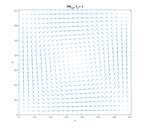
Magnetic field of the TM11 mode of a square of length =
For the mode, the  factor was made to be 100 times less (hence allowing the mode to dissipate much faster). Note from the plot below of the magnetic field that the maximum excitation is expected when the source moves toward the magnetic fields nulls as the next animation shows.
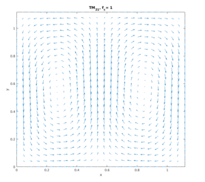
Magnetic field of the TM21 mode.