Emergence of the Dielectric Constant
Introduction
In this article I emphasize the fact that the dielectric constant  encapsulates the behaviour of polarized materials. As has been previously shown, matter senses the fields through Lorentz force. The fields sense matter through charges movements. Here we show how the fields polarize a dielectric (via Lorentz force). In turn, the polarized medium introduces a current proportional to the electric field. Due to this proportionality, we are able to lump the effect of the current into a parameter that we can the dielectric constant .
Microscopic, Macroscopic and Observable quantities
In the following discussion we clearly distinguish between two different scales. The first is the atomic or molecular (Microscopic). This scale is the smallest and represents interactions and quantities defined over distances of the order of the distances between atoms and molecules. The behaviour over such range is hard to quantify, at least within the scope of classical electromagnetism, and may vary wildly from one point to the other. Therefore we are led naturally to the second scale: Macroscopic. Here we consider hundreds or thousands or atoms or molecules. This scale is large enough to permit the wildly changing inter-molecular effects to be averaged out, but at the same time it is small enough when compared to the observer’s scale.
It is of utmost importance to distinguish between these two scales. In a classical electromagnetism theory, the microscopic level is not considered. This means that whenever there is a mention of a point-wise quantity, it is implicitly assumed that this is a macroscopic quantity as defined in the previous paragraph. (The simplest example is the density of matter  . Whenever we speak about density at a point, it assumed that this represents the mass contained in a small (enough) volume surrounding the point. The linear size of the volume element is large enough to include the empty distances between atoms. On the other hand, it is small enough when compared to the observer’s scale.)
Dielectric Materials
For our purpose a dielectric can be thought of as an ensemble of atoms or molecules with positive nuclei and negative orbiting electrons such that with no external electric excitation the positive and negative charge centers coincide. Electrons are distributed around the nuclei in specific orbits with a well defined probability distribution function (i.e, the electron cloud) as dictated by Quantum mechanics. Fig. 1 shows a model of a typical dielectric slab. Upon the application of an electric field  the electron cloud center of charge shifts in a direction opposite to , resulting in a net tiny dipole moment. Note that this shift is a fraction of the atom radius and can be considered infinitesimally small. The dipoles can be represented by the simple model shown in Fig. 1(c) and (d).
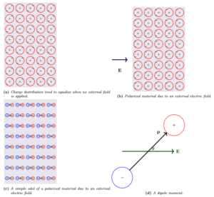
Fig. 1
The dipole moment  is defined as
(1) 
where  is the absolute value of the charge and
  is oriented from the negative to the positive charge. Note that in general there may exist other restoring forces that restrain the dipole moment . This implies that might not be in the same direction as . For simplicity we only consider the case where the is proportional to
(2) 
Since in matter there is a significant large number of dipoles, it is better to use density quantities. The polarization vector  is defined to be the total dipole moment per unit volume. Therefore,
(3) 
where  is known as the electric susceptibility.
Regardless of the source of a polarization vector , we will assume in the next subsection that is given and our task is to calculate the total bounded charge flow crossing some surface  during the time interval
 ![[t_1,t_2]](http://samehelnaggar.ca/wp-content/ql-cache/quicklatex.com-1914a296c1c217138503c71fb7d75fc6_l3.png "Rendered by QuickLaTeX.com") .
.
Bounded charge flow 
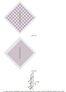
Fig. 2
To understand the effect of polarization, compare the situation where the dipoles of a material are randomly oriented to the one when they are polarized in some direction (Figs. 2(a) and (b)). If we consider that positive charges (nuclei) to be stationary, then the polarization is due to the minute shift of the electron clouds by a distance  . Unlike the case where dipoles are randomly oriented, the net charge crossing a surface is non-zero when the material has a net polarization. Fig. 2(c) highlights a close up view of a polarized material in the vicinity of a surface . Note that dipoles inside the parallelogram result in the cross of charges through the surface, where each dipole’s contribution is precisely . Therefore, the total number of suspended charges is the same as the total number of dipoles
(4) 
where  such that
  is the parallelogram area and
  is the height out of the page. The negative sign emphasizes the fact that negative charges cross the surface. In turn,
  (
( is the length of the interface and
  is the angle between
  and the normal to the surface). Therefore,
(5) 
where  is the area normal to the plane.
So far we have calculated the total charge that crossed the surface as a result of the polarization \mb{P} at some time  . If the polarization changes at another instant
  , the total charge will change. Therefore, the net charge crossing between and in the direction of the area vector becomes
(6) 
where  . The average current over the interval
  is
is
(7) 
where  is the average bounded current flowing through the area
  and
and  is the current density. Over infinitesimal area
  and time interval
  , the macroscopic current density can be found to be
(8) 
From an electromagnetic point of view, (6) encapsulates the effect of the dielectric by showing that a dielectric behaves as source of current. However, this current has a very specific nature: it represents the motion of bounded charges. Maxwell’s equations can be updated to include such source of charge movement. Therefore, Ampere-Maxwell’s equation in its global form becomes
(9) 
where  and
and  represents the current density coming from sources other than polarization.
Update of Gauss’s Law
We already know that
(10) 
where  is all the charge in the volume enclosed by the closed surface . can be divided to two components
  due polarization and other sources. Hence
![\[Q=Q_b+Q_0,\]](http://samehelnaggar.ca/wp-content/ql-cache/quicklatex.com-f16c4b7aedeb458318412a6089a266ec_l3.png "Rendered by QuickLaTeX.com")
where  . ( is the charge left inside the volume. This means that
  .), Therefore,
(11) 